pic
Personal
Website

11b. Introduction to Multithreading

PhD in Economics

Introduction

A correct implementation of multithreading requires a basic understanding of how computers execute instructions. In particular, it's essential to understand this procedure in light of data dependencies: situations where one operation relies on the output of a previous one. If these dependencies aren't properly managed, multithreading could introduce several forms of unsafe code, potentially leading to incorrect results.

This section introduces the preliminary concepts needed to reason about these issues, laying the foundation for the more practical discussions that follow. The emphasis here is on explanation rather than implementation. Accordingly, many of the macros and functions presented will serve only as illustrative examples and won't be reused elsewhere on this website.

Nature of Computations

Operations can be broadly classified based on their data dependency. A dependent operation is one whose outcome is influenced by the result of another operation. In such cases, the order of execution is critical, because changing the sequence can alter the final outcome. In contrast, an independent operation produces the same result, regardless of the order in which it's executed relative to other operations.

The following code gives rise to a dependent or independent operation, based on which values operation B sums.

job_A()  = 1 + 1
job_B(A) = 2 + A

function foo()
    A = job_A()
    B = job_B(A)

    return A,B
end
job_A() = 1 + 1
job_B() = 2 + 2

function foo()
    A = job_A()
    B = job_B()

    return A,B
end

Regardless of their dependency status, operations can be computed either sequentially or concurrently. A sequential procedure involves executing operations one after the other, ensuring each operation completes before the next one begins. Conversely, concurrency allows multiple operations to be processed simultaneously, opening up opportunities for parallel execution.

Like most programming languages, Julia defaults to a sequential execution. This is a deliberate design choice that prioritizes result correctness, as concurrent execution of dependent operations can yield incorrect results if mishandled. The issue arises because concurrency introduces non-determinism in the execution order, which can lead to timing inconsistencies when reading and writing data. A sequential approach precludes this possibility by guaranteeing a predictable order of execution.

Despite its advantages regarding safety, a sequential approach can be quite inefficient for independent tasks: by restricting computations to one at a time, computational resources may go underutilized. In contrast, a simultaneous approach allows for operations to be calculated in parallel, thereby fully utilizing all the available computational resources. This can lead to significant reductions in computation time.

Because most programming languages default to sequential execution, certain nuances of concurrent programming can be difficult to grasp (e.g., concurrency doesn't necessarily imply simultaneity). Such misunderstandings can lead to flawed program design or incorrect handling of concurrent processes. To address this, we next revisit the topic in light of the fundamental concepts of tasks and threads.

Tasks and Threads

When computing an operation, Julia internally defines a set of instructions to be processed. This is achieved through the concept of tasks. For a task to be computed, it must be assigned to a computer thread. Since a single task runs on exactly one thread at a time, the number of threads available on your computer determines how many tasks can be computed simultaneously.

Importantly, each session in Julia starts with a predefined pool of threads, defaulting to a single thread regardless of your computer's hardware. We'll begin by examining the single-threaded case, as it provides a clear basis for understanding concurrency.

To build intuition, consider two workers A and B, whom we'll think of as employees working for a company. B's job consists of performing the same operation continuously for a certain period of time. In the code, this is represented by summing 1+1 repeatedly for one second. For its part, A's job consists of waiting for some delivery, which will arrive after a certain period of time. In the code, this job is represented by performing no computations for two seconds, simulated by calling the function sleep(2).

The following code snippet defines functions capturing each worker's job.

function job_A(time_working)
    sleep(time_working)        # do nothing (waiting for some delivery in the example)

    println("A completed his task")
end
function job_B(time_working)
    start_time = time()

    while time() - start_time < time_working
        1 + 1                  # compute `1+1` repeatedly during `time_working` seconds
    end

    println("B completed his task")
end

Due to the lazy nature of function definitions, these code snippets merely create a blueprint for a set of operations. This implies that no computation is performed. It's only when we call these functions by lines like job_A(2) and job_B(1) that the operations are sent for execution.

To lay bare the internal steps Julia follows for computation, let's adopt a lower-level approach where the function calls job_A(2) and job_B(1) are defined as tasks. As shown below, tasks aren't abstractions to organize our discussion, but actual constructs in Julia's codebase.

A = @task job_A(2)      # A's task takes 2 seconds
B = @task job_B(1)      # B's task takes 1 second

Once a task is defined, the first step for its computation is scheduling it. This means the task is added to the queue of operations awaiting execution by the computer's processor. Then, as soon as a thread becomes available, the machine begins its computation.

Importantly, multiple tasks can be processed concurrently, without implying that they'll be computed simultaneously. Indeed, this is the case in a single-thread session. The distinction can be understood through an analogy with juggling: a juggler manages multiple balls at the same time, but only holds one ball at any given moment. Similarly, multiple tasks can be processed simultaneously, even when only one is actively executing on the CPU.

The implication of this statement is that true parallelism isn't feasible in single-threaded sessions. Nonetheless, concurrency can still improve efficiency through task switching. This is enabled by a task-yielding mechanism: when a task becomes idle (e.g., waiting for input or data), it can voluntarily relinquish control of the thread, allowing other tasks to utilize the thread's time. By fostering a cooperative approach, concurrency ensures plenty of computer resource utilization at any given time.

In the following, we describe this mechanism in more detail.

Sequential and Concurrent Computations

While code is executed sequentially by default, tasks are designed to run concurrently. As a result, to enforce a sequential execution of tasks, we must instruct Julia to run them one at a time. This is achieved by introducing a "wait" instruction immediately after scheduling a task, ensuring that the task completes its calculation before proceeding with the rest of the program.

The code snippet below demonstrates this mechanism by introducing the functions schedule and wait.

A = job_A(2)            # A's task takes 2 seconds
B = job_B(1)            # B's task takes 1 second
Output in REPL
gif
A = @task job_A(2)      # A's task takes 2 seconds
B = @task job_B(1)      # B's task takes 1 second

schedule(A) |> wait
schedule(B) |> wait
Output in REPL
gif
A = @task job_A(2)      # A's task takes 2 seconds
B = @task job_B(1)      # B's task takes 1 second

(schedule(A), schedule(B)) .|> wait
Output in REPL
gif

Note that wait was added even in the concurrent case and after both tasks were scheduled. The purpose is to pause the main program flow until both scheduled tasks have finished, preventing subsequent code from executing prematurely.

The example reveals the benefits of task switching under concurrency: although only one task can run at any moment, task A can yield control of the thread to task B when it becomes idle. In the code, the idle state is simulated by the function sleep, during which the computer performs no operations. Once task A becomes idle, its state is saved, allowing it to eventually resume execution from where it left off. In the meantime, task B can use that thread's processing time, explaining why task B finishes first.

By taking turns efficiently and sharing the single available thread, tasks make the most of the CPU’s processing power. This contrasts with a sequential approach, where task A must finish before moving to the next task. The difference is reflected in their execution times, resulting in 2 seconds for the concurrent approach and 3 seconds for the sequential one.

Examples of idle states emerge naturally in real-world scenarios. For instance, it's common when a program is waiting for user input, such as a keystroke or mouse click. It can also arise when browsing the internet, where the CPU may idle while waiting for a server to send data. Task switching is so ubiquitous in certain contexts that we often take it for granted. For instance, I bet you never questioned whether you could use the computer while a document prints in the background!

Notice, though, that concurrency with a single thread offers no benefits if both tasks require active computations. This is because the CPU would be fully utilized, leaving no chance for task switching. In such cases, the sequential and concurrent approaches are equivalent. In our example, this would occur if task B consisted of computing 1+1 repeatedly, resulting in an execution time of 3 seconds for both approaches.

function job(name_worker, time_working)
    start_time = time()

    while time() - start_time < time_working
        1 + 1                  # compute `1+1` repeatedly during `time_working` seconds
    end

    println("$name_worker completed his task")
end

function schedule_of_tasks()
    A = @task job("A", 2)      # A's task takes 2 seconds
    B = @task job("B", 1)      # B's task takes 1 second

    schedule(A) |> wait
    schedule(B) |> wait
end
Output in REPL
gif
function schedule_of_tasks()
    A = @task job("A", 2)      # A's task takes 2 seconds
    B = @task job("B", 1)      # B's task takes 1 second

    (schedule(A), schedule(B)) .|> wait
end
Output in REPL
gif

Overall, the key insight from this subsection is the underlying procedure outlined: when a task is scheduled, the computer attempts to find an available thread to run it. For concurrency, this implies that starting a session with multiple threads enables parallel code execution. This case is simply referred to as multithreading and explained next in more detail.

Multithreading

Let's revisit the case where both workers A and B perform meaningful computations. The only change introduced is that Julia's session now starts with more than one thread available. For the concurrent approach, we also specify that the tasks are "non-sticky". This technical detail means a task can run on any available thread, not just the one it started on, allowing for more efficient resource allocation.

Once there's more than one thread available, concurrency implies simultaneity. This means each task runs on a different thread, which is why task B finishes first in the following implementation.

function schedule_of_tasks()
    A = @task job("A", 2)                         # A's task takes 2 seconds
    B = @task job("B", 1)                         # B's task takes 1 second

    schedule(A) |> wait
    schedule(B) |> wait
end
Output in REPL
gif
function schedule_of_tasks()
    A = @task job("A", 2) ; A.sticky = false      # A's task takes 2 seconds
    B = @task job("B", 1) ; B.sticky = false      # B's task takes 1 second

    (schedule(A), schedule(B)) .|> wait
end
Output in REPL
gif

Previewing some of the approaches we'll introduce later, let's compare Julia's default implementation (sequential) with a multithreaded one. The macro @spawn, which will be covered in the next section, offers a simple way to run tasks in a multithreaded environment. Essentially, it's equivalent to creating and scheduling a non-sticky task. The following code snippets demonstrate both the default and multithreaded approaches.

function schedule_of_tasks()
    A = job("A", 2)             # A's task takes 2 seconds
    B = job("B", 1)             # B's task takes 1 second
end
Output in REPL
gif
function schedule_of_tasks()
    A = @spawn job("A", 2)      # A's task takes 2 seconds
    B = @spawn job("B", 1)      # B's task takes 1 second

    (A,B) .|> wait
end
Output in REPL
gif

The Importance of Waiting For The Results

Before concluding this section, it's worth stressing a crucial point: you must always instruct your program to wait for operations to complete before proceeding. This holds true even for concurrent computations. Failing to wait may produce incorrect results, even in a single-threaded environment.

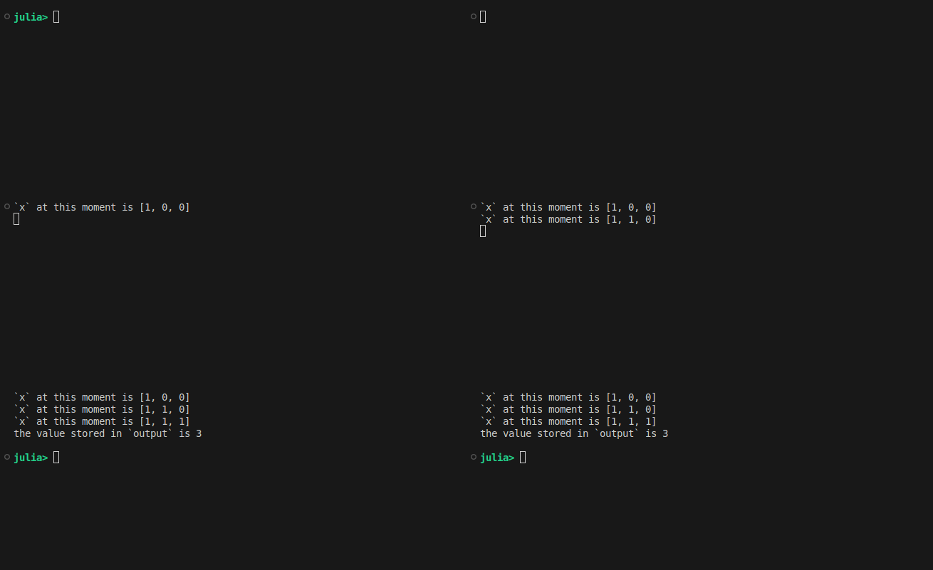
To illustrate this, consider mutating a vector in a single-threaded session, with a one‑second delay for each value update. If we don’t wait for the mutation to finish, any subsequent operation will be based on the vector’s value at the moment it's accessed. This value doesn't necessarily reflect its final mutated state, but merely its value at the moment of reference.

For instance, suppose we seek to mutate the vector x = [0,0,0] into x = [1,2,3]. Let's begin considering Julia’s default sequential execution. This ensures that the mutation completes before continuing with any other operation.

# Description of job
function job!(x)
    for i in 1:3
        sleep(1)     # do nothing for 1 second
        x[i] = 1     # mutate x[i]

        println("`x` at this moment is $x")
    end
end

# Execution of job
function foo()
    x = [0, 0, 0]

    job!(x)          # slowly mutate `x`

    return sum(x)
end

output = foo()
println("the value stored in `output` is $(output)")
Output in REPL
gif

Let's now consider the same implementation but through tasks. In particular, we define a task to perform a mutation as follows.

function job!(x)
    @task begin
        for i in 1:3
            sleep(1)    # do nothing for 1 second
            x[i] = 1    # mutate x[i]

            println("`x` at this moment is $x")
        end
    end
end

The following snippets show the consequences of waiting versus not waiting for the task to complete.

function foo()
    x = [0, 0, 0]

    job!(x) |> schedule             # define job, start execution, don't wait for job to be done

    return sum(x)
end

output = foo()
println("the value stored in `output` is $(output)")
Output in REPL
gif
function foo()
    x = [0, 0, 0]

    job!(x) |> schedule |> wait     # define job, start execution, only continue when finished

    return sum(x)
end

output = foo()
println("the value stored in `output` is $(output)")
Output in REPL
gif

Without a wait call, the main program schedules the mutation task and immediately proceeds to the next line. Since the task contains a sleep instruction, the mutation hasn't yet begun when x is accessed, resulting in the use of its original value [0,0,0]. This demonstrates that properly synchronizing tasks is essential for correctness.