pic pic
Personal
Website

7e. Functions: Type Inference and Multiple Dispatch

PhD in Economics
Code Script
This section's scripts are available here, under the name allCode.jl. They've been tested under Julia 1.11.8.

Introduction

Functions play a central role in Julia to achieving high performance. This role is by design: they have been engineered from the outset to generate efficient machine code. In practice, it means that wrapping code within functions isn't just good programming practice for organizing logic. It's actually necessary to attain fast execution.

However, to fully unlock the power of functions, we must first understand the underlying process of function calls. Essentially, when a function is called, Julia attempts to identify concrete types for its variables, eventually selecting a corresponding computation method. At the heart of the process are three interconnected mechanisms: dispatch, compilation, and type inference. This section will provide a detailed explanation of each.

Variable Scope In Functions

To understand why functions are central to writing high-performance code, recall the variable scope of functions. Local variables consist of function arguments and variables created within the function body. They exist only during the function's execution and are inaccessible from outside. Global variables, on the other hand, refer to any variable defined outside the function and remain accessible throughout program execution.

When code runs inside a function and all its variables are local, the compiler can reason about types, optimize aggressively, and generate efficient machine code. Global variables disrupt this process, as their types and values can change at any time, forcing the compiler to insert dynamic lookups. This process prevents key optimizations, resulting in a substantial performance degradation.

The use of global variables isn't limited to code written in the global scope. It also arises when a function references or writes variables that either aren't passed as arguments or are defined in the function body. As a result, the performance drawbacks from global variables are present in all the following cases.

x   = 2

y   = 3 * x
Output in REPL
julia>
y
6
x   = 2

f() = 3 * x
Output in REPL
julia>
f()
6

Recall that an assignment like x = 2 is shorthand for x::Any = 2, reflecting that global variables default to Any if they aren't explicitly type-annotated. Furthermore, only concrete types can be instantiated, meaning that values can only adopt a concrete type. This is why x::Any shouldn't be interpreted as x having type Any, but rather that x can take on any concrete type that's a subtype of Any. Since Any sits at the top of Julia's type hierarchy, this simply means that x's types are unrestricted.

The unrestricted nature of global variables is precisely what prevents Julia from specializing operations. In our example, x is a global variable, and so the specialization of * is precluded. Specifically, once a global variable is introduced, Julia must consider multiple possible methods for the computation of *, one for each possible concrete type of x. In practice, this leads to code generation with multiple branches, potentially involving type checks, conversions, and memory allocations. The consequence is degraded performance.

The underlying logic for Julia treating global variables as potentially embodying any type and value is that, even if a variable holds some value at a specific moment, the user may reassign it at any point in the program. Note that the performance issues wouldn't completely go away if we had type-annotated x with a concrete type such as x::Int64 = 2. The reason is that many optimizations depend not only on knowing the concrete type of a variable, but also on knowing its value and having a well-defined scope where that value exists. It's only when these assumptions are met that Julia can gain a comprehensive view of all the operations to be performed, creating opportunities for optimizations.

Functions in Julia are designed precisely to provide these guarantees. By enforcing local scope and predictable variable behavior, they enable method specialization and unlock the full range of performance optimizations. Next, we explore the specific steps that Julia takes to achieve this.

Functions and Methods

A function is simply a name that can be associated with different implementations. Each implementation is known as a method. This specifies the function body for a particular combination of argument types and number of arguments. You can inspect the methods associated with a function foo by executing methods(foo).

To illustrate, let's define several methods for the function foo1. Creating a method requires type-annotating the arguments of foo1 during its definition, implemented via the :: operator. In this way, we can set a distinct function body for each unique combination of argument types.

To keep matters simple, let's begin with a scenario where all the methods of foo1 take the same number of arguments, thus differing only in their types.

foo1(a,b)                  = a + b
foo1(a::String, b::String) = "This is $a and this is $b"
Output in REPL
julia>
methods(foo1)
2 methods for generic function "foo1" from Main

julia>
foo1(1,2)
3

julia>
foo1("some text", "more text")
"This is some text and this is more text"

Since foo1(a,b) is equivalent to foo1(a::Any,b::Any), the first method sets the behavior of foo1 for every possible pair of argument types. The second method foo1(a::String, b::String) overrides the function's behavior when both arguments are strings.

The existence of multiple methods explains why the two calls produce different outputs: executing foo1(1, 2) makes use of the first method of foo1, whereas foo1("some text", "more text") triggers the second method.

The example also reveals that methods don't need to perform similar operations. Although it's usually unwise to group unrelated behaviors under a single function name, this capability serves a different purpose. It allows developers to optimize algorithms for specific variable types, which is central to performance-oriented programming. Thus, by reusing the same function name across different implementations, the execution strategy is tailored to each type, while maintaining a consistent interface for users.

Also note that methods don't need to have the same number of arguments. For instance, it's possible to define the following methods for a function foo2.

foo2(x)       = x
foo2(x, y)    = x + y
foo2(x, y, z) = x + y + z
Output in REPL
julia>
methods(foo2)
3 methods for generic function "foo2" from Main

julia>
foo2(1)
1
julia>
foo2(1, 2)
3
julia>
foo2(1, 2, 3)
6

Defining methods with different number of arguments is particularly useful for extending a function's behavior. A prime example is given by the function sum. So far, we've only used its simplest form sum(x), which adds all the elements of a collection x. However, sum also supports additional methods. One of them is sum(<function>, x), where the elements of x are transformed via <function> before being summed.

x = [2, 3, 4]

y = sum(x)          # 2 + 3 + 4
z = sum(log, x)     # log(2) + log(3) + log(4)

Function Calls

Building on our understanding of how functions and methods are defined, let's now analyze the process triggered when a function is called. All our explanations will be based on the following function foo:

foo(a, b) = 2 + a * b
Output in REPL
julia>
foo(1, 2)
4

julia>
foo(3, 2)
8

julia>
foo(3.0, 2)
8.0

Defining a function like foo(a, b) is shorthand for creating a method with the signature foo(a::Any, b::Any). This means the function body applies to every possible combination of argument types.

When we call foo(1, 2), Julia evaluates the expression 2 + a * b by following a well-defined sequence of steps.

The process begins with what's known as multiple dispatch, where Julia selects which method of the function to execute. Importantly, this decision is based solely on the concrete types of the function arguments, not their values. The information on types is then used to select a method, which defines the function body and hence the operations to be performed. This process involves searching through the available methods of foo, eventually choosing the most specific one that matches the concrete types of a and b. The function foo in our example has only the single method foo(a,b) = 2 + a * b. This applies to any argument types, including a::Int64 and b::Int64, and so the corresponding function body is 2 + a * b.

Once the method is chosen, Julia looks for a method instance, which is the compiled version of the method specialized for the signature foo(a::Int64, b::Int64). If such an instance already exists, Julia reuses it immediately to compute foo(1,2). If not, the compiler generates optimized machine code for that specific type combination, caches it for future calls, and then executes it. This on-demand specialization is one of the key reasons Julia can offer a performance that's close to low-level languages.

The following diagram depicts the process unfolded when foo(1,2) is executed.

Multiple Dispatch
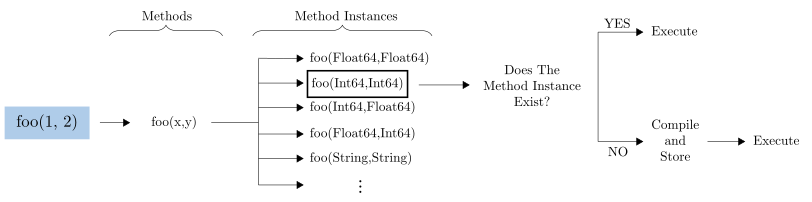

The process outlined has implications for how the language works. In particular, the first time a function is called with a particular combination of concrete types, Julia incurs a time cost to generate specialized code for those types. This initial delay is often referred to as Time To First Plot, a phrase that highlights how noticeable the compilation overhead was in plotting libraries. Starting with Julia 1.9, the ability to precompile packages has improved substantially. As a result, the issue primarily affects user-defined functions and uncommon type combinations that weren't precompiled by packages. In these cases, the user will still experience compilation delays during the first execution.

Note, though, that once Julia compiles a method instance, it caches the resulting code. Consequently, any later call with the same argument types can reuse that cached instance immediately, avoiding the compilation step entirely. In practical terms, it implies that all subsequent function calls with the same concrete types are fast.

The behavior of foo illustrates this process clearly. After evaluating foo(1, 2), Julia has already compiled a method instance for the specific signature foo(a::Int64, b::Int64). Thus, the subsequent call foo(3, 2) is executed immediately using the cached method instance, without any need for recompilation. Instead, the execution of foo(3.0, 2) introduces a new combination of argument types a::Float64 and b::Int64. Because no compiled method instance yet exists for this signature, Julia must generate one before executing the function.

Type Inference

As we indicated, Julia generates the machine code to implement a function during the compilation process. Most considerations for achieving high performance are tied to this step.

Compilation in Julia happens on demand, right at the moment a function is first called with a new set of argument types. The strategy is known as Just-In-Time Compilation (JIT). A key mechanism in it is type inference, whereby the compiler attempts to identify concrete types for all variables and expressions within the function body.

If the compiler succeeds in identifying concrete types, it can specialize instructions for each operation and yield fast code. For instance in the example above with the function foo, type inference involves determining concrete types for 2, a = 1, and b = 2. Since all values have type Int64, the compiler can specialize the computation of 2 + a * b for variables with type Int64. This is the essence behind type stability, which we'll cover extensively in the next chapter.

On the contrary, if the compiler is unable to identify concrete types for some expressions, it must create generic code to accommodate multiple combinations of types. This forces Julia to perform type checks and conversions during runtime, significantly degrading performance.

Below, we provide various remarks about type inference that are worth keeping in mind for next sections.

Functions Themselves Do Not Guarantee The Identification of Concrete Types

Merely placing code inside a function doesn't guarantee that the compiler will identify concrete types for all operations. The following example illustrates this.

x       = [1, 2, "hello"]    # Vector{Any}

foo3(x) = x[1] + x[2]        # type unstable
Output in REPL
julia>
foo3(x)
3

The issue in the example is that x[1] and x[2] come from an object with type Vector{Any}, and so the compiler assigns the type Any to both. This explains why the compiler can't specialize the computation of +. The example also highlights that compilation is exclusively based on types, not values. Thus, the generated code ignores that the actual values are x[1] = 1 and x[2] = 2, which would otherwise reveal their type Int64.

Global Variables Inherit Their Global Type

Type inference is restricted to local variables. Instead, any global variable inherits its type from the global scope. In the following examples, b and d are global variables. Consequently, the compiler defines the type of b as Any and that of d as Number.

a         = 2
b         = 1

foo4(a)   = a * b
Output in REPL
julia>
foo4(a)
2
c         = 2
d::Number = 1

foo4(c)   = c * d
Output in REPL
julia>
foo4(c)
2

Type-Annotating Function Arguments Does Not Improve Performance

The ability of the compiler to identify concrete types is crucial for achieving high performance. This might wrongly suggest that explicitly annotating function arguments is necessary for performance, or at least beneficial. Thanks to type inference, such annotations are actually redundant. In fact, adding them can be counterproductive: type-annotations unnecessarily restrict the types accepted by a function, thus limiting its flexibility and potential applications.

To see how this loss of flexibility plays out, compare the following scripts.

foo5(a, b) = a * b
Output in REPL
julia>
foo5(0.5, 2.0)
1.0

julia>
foo5(1, 2)
2
foo6(a::Float64, b::Float64) = a * b
Output in REPL
julia>
foo6(0.5, 2.0)
1.0

julia>
foo6(1, 2)
ERROR: MethodError: no method matching foo6(::Int64, ::Int64)

The function on the first tab only accepts arguments of type Float64, meaning that even integers are disallowed. By contrast, the function on the second tab also handles Float64 inputs, but additionally allows for other types. This is due to the implicit type annotation Any on the function arguments.

Packages Commonly Type-Annotate Function Arguments
When inspecting code of packages, you may notice that function arguments are often type-annotated. The reason for this isn't related to performance, but rather to ensure that the function is used as intended, safeguarding against inadvertent type mismatches.

For instance, suppose a function that computes theater revenue via nr_tickets * price. In Julia, the operator * not only implements the product of numbers, but also concatenates words when applied to expressions with type String. Without type-annotations, the function could potentially be misused, as exemplified in the first tab below. The second tab precludes this possibility by asserting types.

revenue1(nr_tickets, price) = nr_tickets * price
Output in REPL
julia>
revenue1(3, 2)
6

julia>
revenue1("this is ", "allowed")
"this is allowed"
revenue2(nr_tickets::Int64, price::Number) = nr_tickets * price
Output in REPL
julia>
revenue2(3, 2)
6

julia>
revenue2("this is ", "not allowed")
ERROR: MethodError: no method matching revenue2(::String, ::String)