Generic expressions are represented by <something> (e.g., <function> or <operator>). This is just notation, and the symbols < and > should not be misconstrued as Julia's syntax.
PAGE LAYOUT
If you want to adjust the size of the font, zoom in or out on pages by respectively using Ctrl++ and Ctrl+-. The layout will adjust automatically.
LINKS TO SECTIONS
To quickly share a link to a specific section, simply hover over the title and click on it. The link will be automatically copied to your clipboard, ready to be pasted.
KEYBOARD SHORTCUTS
Action
Keyboard Shortcut
Previous Section
Ctrl + 🠘
Next Section
Ctrl + 🠚
List of Subsections
Ctrl + x
Search
Ctrl + Shift + F
Open All Codes and Outputs in a Post
Alt + 🠛
Close All Codes and Outputs in a Post
Alt + 🠙
TIME MEASUREMENT
When benchmarking, the equivalence of time measures is as follows.
This section's scripts are available here, under the name allCode.jl. They've been tested under Julia 1.11.8.
Introduction
The previous section introduced the basics of multithreading. We highlighted that operations can be computed either sequentially (Julia's default) or concurrently. The latter enables the processing of multiple operations simultaneously, with each of them running as soon as a thread becomes available. When Julia's session is initialized with more than one thread, this determines that computations can be executed on different CPU cores in parallel.
The current section will focus on Julia's native multithreading mechanisms. The topic will span several sections. Our primary goal here is to demonstrate how to write multithreaded code, rather than exploring how and when to apply the technique. We've deliberately structured our explanation in this way to smooth subsequent discussions.
Warning!
While multithreading can offer significant performance advantages, it's not applicable in all scenarios. In particular, multithreading demands extreme caution in handling dependencies between operations, as mismanagement can lead to silent catastrophic bugs.
This is why the section only aims at grasping a basic understanding of parallelism techniques. We'll devote an entire section on thread-unsafe operations.
Enabling Multithreading
Each Julia session is initialized with a given pool of threads available. Since each thread can run a set of instructions independently, the total number of threads determines how many instructions can be processed simultaneously.
By default, Julia runs in single-threaded mode. Consequently, you must configure it to enable multithreading. Importantly, once this configuration is set, the change is permanent: every new Julia session will start with the number of threads you specified.
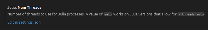
In VSCode or VSCodium, multithreading is enabled by navigating to File > Preferences > Settings. Then, you must search for the keyword threads, which will display the following option:
After selecting Edit in settings.json, add the line "julia.NumThreads": "auto" in the file that opens. The specification auto automatically detects the number of threads supported by your system, typically matching the logical or physical cores of your CPU.
Notice the effects will only take place after a new session is started. To check whether the effects have taken place, run the command Threads.nthreads(). This displays the number of threads available in the running session. Any number greater than one will indicate multithreading is active.
Once a multithreaded session is started, there are several packages available for performing parallel computations. The current section will focus on the capabilities built directly into Julia, which are provided by the Threads package. This package is automatically "imported" in every Julia session, so you can call its functions and macros by prefixing them with Threads. Alternatively, you can load the package with using, which lets you use its macros and functions without qualification.
# package `Threads` is automatically imported when you start a Julia session

Threads.nthreads()
Output in REPL
24
using Base.Threads      # or `using .Threads`

nthreads()
Output in REPL
24
Warning! - Loaded Package
All the scripts below assume that you've executed using Base.Threads. This allows direct access to macros like @spawn.
Task-Based Parallelism: @spawn
The first approach to parallel execution we introduce is the macro @spawn. By prefixing an expression with @spawn, Julia creates a (non-sticky) task that's immediately scheduled for execution. If a thread is available, the task begins running right away.
Unlike other parallel programming approaches we'll examine later, @spawn requires explicit instructions to wait for task completion. The method for doing so depends on the nature of the task output.
The fetch function is required when tasks return a result. It serves a dual purpose: it waits for a task to complete and returns the task's output. Since parallel programs involve multiple spawned tasks, fetch should be broadcast over a collection containing all tasks.
The following example demonstrates fetch with two spawned tasks.
x = 2

function foo(x)
    a      = x * -2
    b      = x *  2

    a,b
end
Output in REPL
julia>
foo(x)
(-4, 4)
x = 2

function foo(x)
    task_a = @spawn x * -2
    task_b = @spawn x *  2

    a,b    = fetch.((task_a, task_b))
end
Output in REPL
julia>
foo(x)
(-4, 4)
Note that fetch takes tasks as input. This is why it's important to distinguish between task_a and a:
task_a denotes the task creating the vector a (i.e., the task itself),
a refers to the vector created (i.e., the task's output).
Alternatively, for tasks that perform actions without returning a value, we can use either the function wait or the macro @sync. The function wait works analogously to fetch, except that it doesn't return any value. For its part, the macro @sync requires enclosing all the operations to be synchronized between the keywords begin and end.
To illustrate, consider a mutating function. Such functions are suitable examples for both cases, since they don't return a value.
x = rand(10)
y = rand(10)

function foo!(x,y)
    @. x = -x
    @. y = -y
end
x = rand(10)
y = rand(10)

function foo!(x,y)
    task_a = @spawn (@. x = -x)
    task_b = @spawn (@. y = -y)

    wait.((task_a, task_b))
end
x = rand(10)
y = rand(10)

function foo!(x,y)
    @sync begin
        @spawn (@. x = -x)
        @spawn (@. y = -y)
    end
end
Multithreading Overhead
To see @spawn in action, let's calculate both the sum and the maximum of a vector x. Their computation will be implemented following a sequential and a simultaneous approach. These implementations will reveal that the total runtime of the sequential procedure is essentially the sum of the individual runtimes. In contrast, thanks to parallelism, the runtime under multithreading is roughly equivalent to the longer of the two computations.
x = rand(10_000_000)

function non_threaded(x)
    a           = maximum(x)
    b           = sum(x)

    all_outputs = (a,b)
end
Output in REPL
julia>
@btime maximum($x)
7.494 ms (0 allocations: 0 bytes)
julia>
@btime sum($x)
3.041 ms (0 allocations: 0 bytes)
julia>
@btime non_threaded($x)
10.666 ms (0 allocations: 0 bytes)
x = rand(10_000_000)

function multithreaded(x)
    task_a      = @spawn maximum(x)
    task_b      = @spawn sum(x)

    all_tasks   = (task_a, task_b)
    all_outputs = fetch.(all_tasks)
end
Output in REPL
julia>
@btime maximum($x)
7.494 ms (0 allocations: 0 bytes)
julia>
@btime sum($x)
3.041 ms (0 allocations: 0 bytes)
julia>
@btime multithreaded($x)
7.631 ms (13 allocations: 1.031 KiB)
Although the multithreaded runtime is close to the maximum of the individual runtimes, the equivalence isn't exact. The reason is that multithreading introduces overhead due to the creation, scheduling, and synchronization of tasks. A practical consequence of this behavior is that multithreading can actually be counterproductive for small workloads, where the overhead can outweigh any performance gains.
To make this trade-off concrete, let's compare the execution times of a sequential and multithreaded approach for different sizes of x. In the examples, multithreading is only advantageous for sizes greater than 100,000, with the single-threaded approach dominating otherwise. The high threshold illustrates just how significant the overhead can be relative to the actual work performed.
x_small  = rand(    1_000)
x_medium = rand(  100_000)
x_big    = rand(1_000_000)

function foo(x)
    a           = maximum(x)
    b           = sum(x)

    all_outputs = (a,b)
end

 Home
Home Chapters
 Links
Links BOOK in PDF