Generic expressions are represented by <something> (e.g., <function> or <operator>). This is just notation, and the symbols < and > should not be misconstrued as Julia's syntax.
PAGE LAYOUT
If you want to adjust the size of the font, zoom in or out on pages by respectively using Ctrl++ and Ctrl+-. The layout will adjust automatically.
LINKS TO SECTIONS
To quickly share a link to a specific section, simply hover over the title and click on it. The link will be automatically copied to your clipboard, ready to be pasted.
KEYBOARD SHORTCUTS
Action
Keyboard Shortcut
Previous Section
Ctrl + 🠘
Next Section
Ctrl + 🠚
List of Subsections
Ctrl + x
Search
Ctrl + Shift + F
Open All Codes and Outputs in a Post
Alt + 🠛
Close All Codes and Outputs in a Post
Alt + 🠙
TIME MEASUREMENT
When benchmarking, the equivalence of time measures is as follows.
This section's scripts are available here, under the name allCode.jl. They've been tested under Julia 1.11.9.
Introduction
This section introduces standard tools for benchmarking code performance. Our book reports results based on the BenchmarkTools package, which is currently the most mature and reliable option in the Julia ecosystem. That said, the newer Chairmarks package has demonstrated notable improvements in execution speed compared with BenchmarkTools. I recommend adopting Chairmarks once it's achieved sufficient stability and adoption within the community.
To set the stage, we'll start by addressing some key points for interpreting benchmark results. We'll also look at Julia's built-in @time macro, whose limitations explain why BenchmarkTools and Chairmarks should be used instead.
Time Metrics
Julia uses the same time metrics described below, regardless of whether you use BenchmarkTools or Chairmarks. For quick reference, these metrics can be accessed at any point in the left bar under "Notation & Hotkeys".
Unit
Acronym
Measure in Seconds
Seconds
s
1
Milliseconds
ms
\(10^{-3}\)
Microseconds
μs
\(10^{-6}\)
Nanoseconds
ns
\(10^{-9}\)
Alongside execution times, each package also reports the amount of memory allocated on the heap, typically referred to simply as allocations. These allocations can play a major role in overall performance, and usually indicate suboptimal coding practices. As we'll explore in later sections, monitoring allocations tends to be crucial for achieving high performance.
"Time to First Plot"
The expression "Time to First Plot" refers to a side effect of how Julia operates: the first time you run a function with a specific signature, Julia generates low-level machine instructions to carry out the function's operations. This process of translating human-readable code into machine-executable instructions is called compilation. Unlike many other programming languages, Julia relies on a just-in-time (JIT) compiler, meaning code is compiled on-the-fly when a function is first executed. This compilation process is fundamental to how the language achieves high performance and will be thoroughly covered in upcoming sections.
Nonetheless, the practical impact of this compilation latency has changed significantly with recent developments. Thanks to improvements in the precompilation system (particularly since Julia 1.9), a vast majority of package functions are now pre-compiled before you run code. Consequently, the "compilation penalty" in a new session mainly affects functions defined by the user or novel combinations of argument types that the precompilation doesn't cover. Once a function is compiled, its machine code is cached, making all subsequent calls faster.
The latency varies significantly across functions. While it may be imperceptible for simple operations, it can still be noticeable when triggering a chain of user-defined methods or write complex operations. This explains the origin of the term "Time to First Plot", since drawing the first plot during a session was taking several seconds.
Warning!
While precompilation has reduced the "Time-to-First-Plot" latency, it hasn't changed the JIT compilation model. Understanding that Julia compiles specialized machine code for your specific types remains crucial for writing performant Julia code.
@time
Julia comes with a built-in macro called @time, allowing you to get a quick sense of an operation's execution time. The results provided by this macro, nonetheless, suffer from several limitations that make it unsuitable for rigorous benchmarking.
First, a measurement based on just a single execution is often unreliable, as runtimes can fluctuate significantly due to background processes on your computer. Second, if that run represents a function's first call, the measurement will include compilation overhead. The extra time Julia spends generating machine code inflates the reported runtime, making it unrepresentative of subsequent calls.
Moreover, while running @time multiple times can address these issues, the macro still has a major flaw when used for rigorous benchmarking: it evaluates code in the global scope. We'll show in upcoming sections that non-constant global variables have a marked detrimental effect on performance. Consequently, the time reported doesn't accurately reflect how the function would perform in practice.
The following example illustrates the use of @time, highlighting the difference in execution time between the first and subsequent runs.
x = 1:100

@time sum(x)         # first run                     -> it incorporates compilation time
@time sum(x)         # time without compilation time -> relevant for each subsequent run
A more reliable alternative for measuring execution time is provided by BenchmarkTools. This addresses the shortcomings of @time in several ways.
First, it reduces result variability by running operations multiple times and providing summary statistics. It also measures the execution time of functions without compilation latency, since the package discards the first run for the reported timing. Additionally, the package allows users to explicitly control variable scope: by prefixing function arguments with the $ symbol, these are treated as local variables during a function call.
The package offers two macros, depending on the level of detail required: @btime, which only reports the minimum time, and @benchmark, which provides detailed statistics. Below, we demonstrate their use.
using BenchmarkTools

x = 1:100
@btime sum($x)        # provides minimum time only
Output in REPL
2.314 ns (0 allocations: 0 bytes)
using BenchmarkTools
x = 1:100
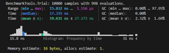
@benchmark sum($x) # provides more statistics than `@btime`
Output in REPL
In upcoming sections, we'll exclusively benchmark functions. This means that you should always prefix the function arguments with $. Omitting$will lead to inaccurate results, including incorrect reports of memory allocations.
The following example demonstrates the consequence of excluding $, where the runtimes reported are higher than the actual runtime.
using BenchmarkTools
x = rand(100)

@btime sum(x)
Output in REPL
14.465 ns (1 allocation: 16 bytes)
using BenchmarkTools
x = rand(100)

@btime sum($x)
Output in REPL
6.546 ns (0 allocations: 0 bytes)
Package "Chairmarks"
A new alternative for benchmarking code is the Chairmarks package. Its notation closely resembles that of BenchmarkTools, with the macros @b and @be providing a similar functionality to @btime and @benchmark respectively. The main benefit of Chairmarks is its speed, as it can be orders of magnitude faster than BenchmarkTools.
As with BenchmarkTools, measuring the execution time of functions appropriately requires prepending function arguments with $.
using Chairmarks
x = rand(100)

display(@b sum($x))        # provides minimum time only
Output in REPL
6.550 ns
using Chairmarks
x = rand(100)

display(@be sum($x))       # analogous to `@benchmark` in BenchmarkTools
Output in REPL
Benchmark: 3856 samples with 3661 evaluations
 min    6.679 ns
 median 6.815 ns
 mean   6.785 ns
 max    14.539 ns
Remark On Random Numbers For Benchmarking
When comparing the performance of different methods, we must ensure that our measurements aren't skewed by variations in the input data. This implies each approach must be tested using the exact same set of values. This guarantees that differences in execution time can be attributed solely to the efficiency of the method itself, rather than to a change in the inputs.
Such consistency can be achieved by using random number generators. They rely on a random seed, which is an arbitrary starting point that dictates the entire sequence of values to be produced. By setting the same seed before each test, we can generate identical deterministic sequences of random numbers across multiple runs. Importantly, any arbitrary number can be used for the seed. The only requirement is that the same number is employed, so that you replicate the exact same set of random numbers.
Random number generation is provided by the package Random. Below, we demonstrate its use by setting the seed 1234 before executing each operation. Note, though, that any other number could be used.
using Random

Random.seed!(1234)      # 1234 is an arbitrary number, use any number you want
x = rand(100)

Random.seed!(1234)
y = rand(100)           # identical to `x`
using Random

Random.seed!(1234)      # 1234 is an arbitrary number, use any number you want
x = rand(100)


y = rand(100)           # different from `x`
For presentation purposes, code snippets in this book will omit the lines dedicated to setting the random seed. While adding these code lines is essential for ensuring reproducibility, their inclusion in every example would create unnecessary clutter. Below, we illustrate the code that will be displayed throughout the book, along with the actual code executed.
using Random
Random.seed!(123)

x = rand(100)

y = sum(x)
# We omit the lines that seet the seed


x = rand(100)

y = sum(x)
Benchmarks In Perspective
When evaluating approaches for performing a task, execution times are often negligible, typically on the order of nanoseconds. Yet, this doesn't mean that the choice of method is without practical consequence.
While it's true that operations in isolation may have an insignificant impact on a program's overall runtime, the relevance of benchmarks emerges when these operations are performed repeatedly. This includes cases where the operation is called in a for-loop or embedded in iterative computations (e.g., solving systems of equations or optimizing functions). In these situations, small differences in timing are amplified, as they are replicated hundreds, thousands, or even millions of times.
An Example
To illustrate this matter, let's consider a specific example. Suppose we want to double each element of a vector x, and then calculate their sum. In the following, we'll compare two different approaches to accomplish this task. Both methods produce the same result.
The first method will be based on sum(2 .* x), with x treated as a global variable. As we'll discuss in later sections, this approach is inefficient. A more performant alternative is given by sum(a -> 2 * a, x), where x is passed as a function argument. The measured runtimes of each approach are as follows.
x      = rand(100_000)

foo()  = sum(2 .* x)
Output in REPL
35.519 μs (5 allocations: 781.37 KiB)
x      = rand(100_000)

foo(x) = sum(a -> 2 * a, x)
Output in REPL
6.393 μs (0 allocations: 0 bytes)
The results reveal that the second approach achieves a significant speedup, requiring less than 15% of the time consumed by the slower method. However, even the "slow" approach is remarkably fast when interpreted in absolute terms, completing in under 0.0001 seconds.
This pattern will be recurring in our benchmarks, where execution times are often negligible. In such cases, the relevance of our conclusions depends heavily on context. If the operation is performed only once, readability should guide the choice of implementation. Instead, if the operation is executed repeatedly, small performance differences accumulate and might become meaningful, making the faster approach a more suitable choice.
To make this point concrete, let's place these functions inside a for-loop that runs 100,000 times. Since our sole goal is to repeat the operation, the iteration variable itself plays no role. In such cases, it's a common practice to employ a throwaway variable: a placeholder that exists only to satisfy syntax requirements, without ever being referenced. This convention signals to other programmers that the variable's value can be safely ignored. In our example, _ serves this purpose within the for-loop. It reflects that each iteration performs exactly the same operation, without depending on the for-loop index.
x      = rand(100_000)
foo()  = sum(2 .* x)

function replicate()
   for _ in 1:100_000
      foo()
   end
end
Output in REPL
5.697 s (500000 allocations: 74.52 GiB)
x      = rand(100_000)
foo(x) = sum(a -> 2 * a, x)

function replicate(x)
   for _ in 1:100_000
      foo(x)
   end
end
Output in REPL
677.130 ms (0 allocations: 0 bytes)
The example starkly reveals the consequences of calling these functions within a for-loop. The execution time of the slow version now jumps to more than 5 seconds, while the fast version finishes in under one second. Such a stark contrast underscores the importance of optimizing functions that are executed repeatedly: even seemingly minor improvements can accumulate into pronounced performance gains.

 Home
Home Chapters
 Links
Links BOOK in PDF