-
 Home
Home
-
 Chapters
-
Introduction
This section will formally define type stability, additionally reviewing tools for verifying the property. In the next section, we'll start the coverage of type stability applied to specific objects.
An Intuition
Previously, we've described the process that unfolds when a function is called. To recap, consider a function
foo(x) = x + 2and a variableawith a specific value assigned. To emphasize that the process depends on types rather than values, we won't explicitly statea's value.When we call
foo(a), Julia must compile a method instance to computea + 2. This process involves creating machine code to calculatea + 2, given the concrete types inferred ofaand2. The resulting instructions are then stored, making them readily available for any subsequent callfoo(b)wherebhas the same concrete type asa.To understand the factors influencing performance, it's essential to distinguish between two distinct phases in a function call: compilation time and runtime. Compilation time takes place when a method instance is created. This entails the generation of machine code, based on the concrete types inferred. Importantly, this process involves no computations, and only takes place during initial function calls. For its part, runtime refers to the moment when the code instructions are actually run. Unlike compilation time, this involving the execution of the compiled code, and occurs every time an operation is computed.
Type Stability and Performance
The key to generating fast code lies in the information available to the compiler during the compilation stage. This is primarily gathered through type inference, where Julia determines the specific type of each variable and expression involved. When the compiler can accurately predict a single concrete type for the function's output, we say that the function call is type stable.
Operationally, the definition implies that the compiler must infer unique concrete types for each expression involved. If the condition is met, the compiler will be able to specialize the computation approach, resulting in fast execution. Essentially, the compiler has sufficient information to determine a straight execution path, thus avoiding unnecessary type checks and dispatches at runtime.
In contrast, type-unstable functions generate code that must accommodate multiple possibilities, with instructions for each possible combination of unique concrete types. This results in additional overhead during runtime, where Julia dynamically gathers type information and perform extra calculations based on this new information. The consequence is a pronounced deterioration in performance.
 Type Stability is a Property of Functional Calls It's common to describe a function as "type stable". Nevertheless, it's not the function itself that is type stable, but rather its calls for given concrete types. The distinction is crucial in practice, as a function can exhibit type stability for certain input types but not others.
An Example
To observe type stability in action, let's consider the following example.
Although both operations are ultimately reduced to computing
1 + 2, the method implemented in each case differs. The first approach in particular is faster, because its computations are based on a type-stable function call.Specifically, the output
x[1] + x[2]in the first can be deduced to beInt64, thus satisfying the definition of type stability. The feature reflects thatx[1]andx[2]are identified asInt64, and so the compiler can generate code specialized to this type. This fast isn't only relevant for the example considered, as the code will apply to any callsum(y)withyhaving typeVector{Float64}.In contrast, the second tab defines a type-unstable function call:
xhas typeVector{Any}, making it impossible to predict a unique concrete type forx[1] + x[2], given the information onx's type. This reflects thatx[1]andx[2]may embody any concrete type that is a subtype ofAny. Consequently, the compiler creates code with numerous conditional statements, where each branch states how to computex[1] + x[2]for each possible type (e.g.Int64,Float64,Float32, etc.). This results in compiled code that is slow, as it'll require extra work during runtime. Moreover, the degraded performance will be incurred for every callsum(y)whereyhas typeVector{Any}.
Remark Julia's developers are continuously improving the compiler, solving and mitigating the impact of certain type instabilities. In fact, numerous operations that were type unstable in older releases are now type stable. This entails that type stability should be viewed as a dynamic aspect of the language.Checking for Type Stability
While slower execution can serve as an indication of type instability, there are more formal and reliable mechanisms to determine this. One such mechanism is the
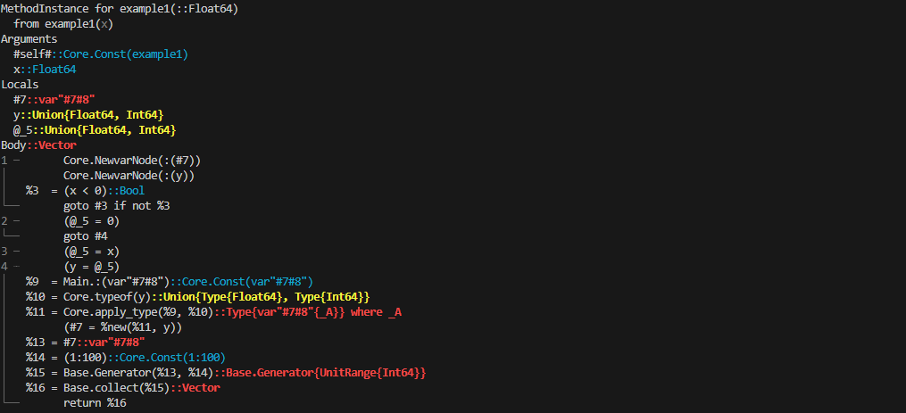
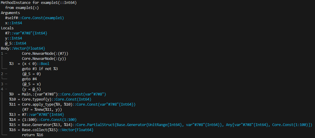
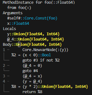
@code_warntypemacro, which reports all the types inferred during a function call.To illustrate its usage, consider a function that defines
yas a transformation ofx, and then usesyto perform some operation.The output of
@code_warntypecan be difficult to interpret. Nonetheless, the addition of colors facilitates its understanding:If all lines are blue, the function is type stable. This means that Julia can identify a unique concrete type for each variable.
If at least one line is red, the function is type unstable. It reflects that one variable or more could potentially adopt multiple possible types.
Yellow lines indicate type instabilities that the compiler can handle effectively, in the sense that they have a reduced impact on performance. As a rule of thumb, you can safely ignore them.
 Warning! Throughout the website, we'll refer to type instabilities as those indicated by a red warning exclusively. Yellow warnings will be mostly ignored.
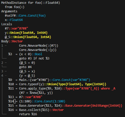
In the provided example, the compiler attempts to infer concrete types. This is by identifying two pieces of information based on
x's concrete type:the type of
y,the type of
y * iwithihaving typeInt64, which implicitly defines the type of[y * i for i in 1:100].
The example clearly demonstrates that the same function can be type stable or unstable depending on the types of its inputs:
foois type stable whenxhas typeInt64, but type unstable whenxisFloat64.In the scenario where
x = 1, the compiler infers for i) thatycan be equal to either0orx. Since both0and1are of typeInt64, the compiler identifies a unique type fory, which isInt64. Regarding ii),y * ialso yields anInt64, as bothiandyhave typeInt64. This establishes that[y * i for i in 1:100]is of typeVector{Int64}. Consequently,foo(1)is type stable, enabling Julia to invoke a method specialized to integers.As for
x = 1.0, the information for i) is thatycould be either0or1.0. As a result, the compiler is unable to infer a unique type fory, which can possibly adopt a value with typeInt64orFloat64. The macro@code_warntypereflects this by identifyingyas having typeUnion{Float64, Int64}. This ambiguity impacts ii), with the compiler unable to specialize and forced to consider an approach that handlesUnion{Float64, Int64}. Overall,foo(1.0)is type unstable, which has a detrimental impact on performance.
Remark The conclusions regarding type stability would've remained the same if we had considered, for instance,foo(-2)orfoo(-2.0). This is because the compilation process relies on information about types, not values. This means that the type stability depends on whetherxhas typeInt64orFloat64, regardless of its actual value.Yellow Warnings May Turn Red
Not all type instabilities have the same impact on performance, and their severity is ultimately indicated through a yellow or red warning. Yellow warnings, which are relatively minor, typically result from isolated computations that Julia can handle effectively. However, if these operations are repeated within a for-loop, they may escalate into more serious performance issues, thus triggering a red warning. The following example demonstrates a scenario like this.
The yellow warning comes from the possibility of
y * 2returning aFloat64orInt64value. However, this operation is computed only once and consists of two types that the compiler can manage well. Instead, the second tab needs to handle a vector with multiple elements created throughy * i, without knowledge ofy's type. This results in a red warning.It's worth remarking, though, that not all yellow warnings necessarily lead to a red one when incorporated into a for-loop. In fact, this doesn't occur in the third tab, where the for-loop doesn't involve a vector. This reinforces the idea that not all type instabilities are equally detrimental.
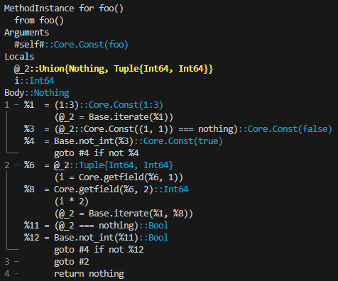
For-Loops and Yellow Warnings When running a for-loop, a yellow warning will always appear even if the operation is type stable. Nevertheless, the warning can be safely ignored, as it merely reflects how iterates work: they return a tuple when there are still remaining elements, or the valuenothingwith typeNothingwhen the sequence is exhausted.For-Loop
function foo()
    for i in 1:100
        i
    end
end
Output in REPLjulia>@code_warntype foo()