Julia 1.9, and each new version is reducing this overhead even further. -
 Home
Home
-
 Chapters
-
Introduction
This section presents standard tools for benchmarking code. Our website in particular will provide results based on the package
BenchmarkTools, which is currently the most mature and reliable option. Nonetheless, the newerChairmarkspackage has shown impressive speed gains. Once it's been around enough to uncover potential bugs, I'd recommend it as the default option.Time Metrics
Regardless of the package employed, Julia uses the same time metrics described below. These metrics can be accessed at any time in the left bar, under "Notation & Hotkeys".
Unit Acronym Measure in Seconds Seconds s1 Milliseconds ms\(10^{-3}\) Microseconds μs\(10^{-6}\) Nanoseconds ns\(10^{-9}\)
All packages additionally provide information about memory allocations on the heap, which are simply referred to as allocations. Their relevance will be explained in the upcoming sections. Basically, they influence performance and potentially hint suboptimal coding.
"Time to First Plot"
The expression "Time to First Plot" refers to a side effect of how the Julia language works: in each session, the first function call is slower than the subsequent ones. This arises because Julia compiles code during its initial run, as we'll explain more thoroughly in the next sections.
This overhead isn't a major hindrance when working on a large project, since the penalty will be incurred only once. However, it determines that Julia may not be the best option when you simply aim to perform a rapid analysis (e.g., run one regression or draw a graph to quickly unveil a relation).
The speed of the first run varies significantly. While it may be imperceptible in some cases, it can be noticeable in others. For instance, I bet you didn't notice that running
sum(x)for the first time in your code was slower than the subsequent runs! On the contrary, drawing high-quality plots can take up to 15 seconds, explaining where the term "Time to First Plot" comes from. [note] The time indicated is forPlots, the standard package for the task. This is a metapackage bundling several plotting libraries. Some of these libraries are relatively fast, requiring less than 5 seconds for rendering the first figure. Warning! The time-to-first-plot issue has been reduced significantly since
@time
Julia comes with a built-in macro called
@timeto measure the execution time of a single run. The results provided by this macro, nonetheless, suffer from two significant limitations. First, the timing provided is volatile and unreliable, as it only considers a single execution. Furthermore, considering the time-to-first-plot issue, the initial timing will incorporate compilation time, and hence it's unrepresentative of the subsequent calls. Taking this into account, you should always execute@timeat least twice. The following illustrates its use, making it clear that the first run includes compilation time.@time
x = 1:100

@time sum(x)         # first run                     -> it incorporates compilation time
@time sum(x)         # time without compilation time -> relevant for each subsequent run
Output in REPL0.003763 seconds (2.37 k allocations: 145.109 KiB, 99.11% compilation time) 0.000005 seconds (1 allocation: 16 bytes)Package "BenchmarkTools"
A better option for measuring execution time is provided by the package
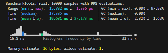
BenchmarkTools. This reports times based on repeated computations of the operation, thus improving accuracy.It can be called through either the macro
@btime, which only reports the minimum time, or through the macro@benchmark, which provides a more detailed analysis. Both macros discard the time of the first call, thus excluding compilation time from the results.Notice that both macros append the symbol
$to the variablex. The notation is necessary to indicate thatxshouldn't be interpreted as a global variable, as occurs when when a variable is passed to a function. As we'll exclusively benchmark functions, you should always add$to each variable—omitting$would lead to inaccurate results.The following example demonstrates the consequence of excluding
$, wrongly reporting higher times than they really are. [note] In fact,sum(x)doesn't allocate memory, unlike what's reported without$.Package "Chairmarks"
A recent new alternative to benchmarking code is given by the package
Chairmarks. Its notation is quite similar toBenchmarkTools, with the macros@band@beproviding a similar functionality to@btimeand@benchmarkrespectively. However,Chairmarksis orders of magnitude faster.Remark On Random Numbers Used On The Website
In the upcoming sections, we'll identify efficient approaches for computing an operation. The tests will be executed relying on random numbers. To eliminate any possible bias, all of them will be based on the same random numbers, which is achieved by specifying a random seed. By doing so, the random number generator produces the same sequence of random numbers every time we execute the program.
The creation of random numbers is given by the package
Random, which requires specifying a seed. You can use any arbitrary number for setting the seed, and ensure that the same seed is established before executing each operation.When any code snippet on this website includes random numbers, we'll exclude the lines setting the random seed. For instance, below we demonstrate what we'll show versus the actual code executed.
Benchmarks In Perspective
In the upcoming chapters, we'll be evaluating approaches for performing a task. Most of the time, the differences in time will be negligible, possibly in the ballpark of nanoseconds. This could mislead us into thinking that the method chosen lacks any practical implication.
It's true that operations in isolation usually have an insignificant impact on runtime. However, the relevance of our benchmarks lies in scenarios where these operations are performed repeatedly. This includes cases where the operation is called in a for-loop, or in iterative procedures (e.g,. solving systems of equations or the maximization of a function). In these situations, small differences in timing are amplified, as they're replicated multiple times.
An Example
Let's illustrate the practical usage of benchmarks by considering a concrete case. Suppose we seek to double each element of
xand then sum them. We'll compare two approaches for this task.The first method will be based on
sum(2 .* x), wherexwill enter into the computation as a global variable. As we'll discuss in later sections, this approach is relatively inefficient. A more efficient alternative is given bysum(a -> 2 * a, x), withxpassed as a function's argument. Aside what this function specifically does, what matters is that it produces the same result as the baseline approach, but implementing a different technique.The runtime of each approach is as follows.
The results reveal that the most efficient approach achieves a significant speedup, taking less than 15% of the slowest approach's time. However, in absolute terms, the "slow" approach is already fast enough, taking less than 0.0001 seconds.
Most of our benchmarks will feature a similar pattern, where absolute times are negligible. In this context, the relevance of the conclusions hinge on the characteristics of our work. If the operation will be called once in isolation, you should prioritize readability and choose the approach most suitable in this regard. On the contrary, if the operation will be performed repeatedly, you should consider that small differences will compound and become significant.
To demonstrate this point, let's call these functions in a for-loop with 100k iterations.
The symbol
_is a programming convention to denote "throwaway" variables. They represent variables solely included to satisfy the syntax of an operation, and their value isn't actually used. In our case, it reflects that each iteration is performing the same operation for benchmark purposes.The example starkly reveals the consequences of calling the function within a for-loop. The execution time of the slow version balloons to more than 20 seconds now, while the fast version does it in under one second. Overall, this unveils the relevance of optimizing functions with repeated or intensive operations, where even slight improvements can have a substantial impact on performance.